Invention for Quantum deep learning

Invented by Nathan Wiebe, Krysta Svore, Ashish Kapoor, Microsoft Technology Licensing LLC
First, it is important to understand what quantum deep learning is and how it works. Quantum computing is a type of computing that uses quantum bits (qubits) instead of classical bits to perform calculations. These qubits can exist in multiple states simultaneously, which allows quantum computers to perform certain calculations much faster than classical computers. Deep learning, on the other hand, is a type of machine learning that uses artificial neural networks to analyze and process data. By combining these two technologies, quantum deep learning aims to create more powerful and efficient algorithms for data analysis.
The market for quantum deep learning is still in its early stages, but it is already showing signs of significant growth. According to a report by MarketsandMarkets, the global quantum computing market is expected to grow from $472 million in 2021 to $1.7 billion by 2026, at a compound annual growth rate (CAGR) of 29.04%. While quantum deep learning is just a small part of this market, it is expected to play a significant role in driving its growth.
One of the main drivers of the market for quantum deep learning is the increasing demand for more powerful and efficient data analysis tools. With the explosion of data in recent years, traditional computing methods are no longer sufficient to process and analyze this data in a timely and accurate manner. Quantum deep learning has the potential to overcome these limitations and provide faster and more accurate insights into complex data sets.
Another factor driving the market for quantum deep learning is the increasing investment in research and development in this field. Many tech companies and research institutions are investing heavily in quantum computing and deep learning, and the combination of these two technologies is seen as a promising area for innovation. This investment is expected to drive the development of new quantum deep learning algorithms and applications, which will in turn drive the growth of the market.
Despite its potential, there are still some challenges that need to be overcome for quantum deep learning to reach its full potential. One of the main challenges is the lack of practical applications for this technology. While there are some promising use cases for quantum deep learning, such as drug discovery and financial modeling, these applications are still in the early stages of development. Another challenge is the high cost of quantum computing hardware, which limits the accessibility of this technology to smaller companies and research institutions.
In conclusion, the market for quantum deep learning is still in its early stages, but it is expected to grow significantly in the coming years. With the increasing demand for more powerful and efficient data analysis tools, and the growing investment in research and development in this field, quantum deep learning has the potential to revolutionize the way we process and analyze data. While there are still some challenges that need to be overcome, the future looks bright for this exciting new technology.

The Microsoft Technology Licensing LLC invention works as follows
Boltzmann machines can be trained by using an objective function, which is evaluated through sampling quantum states that are close to Gibbs states. The objective function is produced using classical processing, while the approximate Gibbs states are based on biases and weights that have been refined utilizing the sample results. In some cases, amplitude estimates are used. “A combined classical/quantum computing system produces weights and biases suitable for the classification of shapes, among other applications.

Background for Quantum deep learning
Deep learning is a relatively recent paradigm in machine learning. It has had a significant impact on the way that classification, inference, and artificial intelligence (AI), tasks are performed. Deep learning was developed on the premise that to achieve sophisticated AI tasks such as language or vision, it might be necessary to use abstractions rather than raw data. In order to train an inference engine to detect a vehicle, it might decompose a raw image into simple shapes. These shapes can form the first abstraction layer. These shapes can be combined to form higher-level abstract objects, such as wheels or bumpers. This abstract data is used to determine whether or not an image is a car. This process can involve several levels of abstraction.
Deep learning techniques have shown remarkable improvements, such as a relative reduction of error rates up to 30% on many typical speech and vision tasks. Deep learning techniques can sometimes be as good as humans at matching faces, for example. Currently, conventional classical deep learning techniques are used in speech models and search engines. Machine translation and deep imaging understanding (i.e. image to text representation) are also applications.
Existing methods of training deep belief network use contrastive divergence appsroximations to build the network layer-by-layer. This is a costly process for deep networks and relies on the validity the contrastive divergence method. It also prevents the use intra-layer connections. In some cases, the contrastive divergence method is not applicable. Contrastive divergence methods also cannot train an entire graph in one go and must be trained in layers. This is expensive and lowers the quality. Finaly, more crude approximations will be needed to train the full Boltzmann Machine, which may have connections between hidden and visible units, and could limit the quality found in the algorithm. “We need to find ways to overcome these limitations.
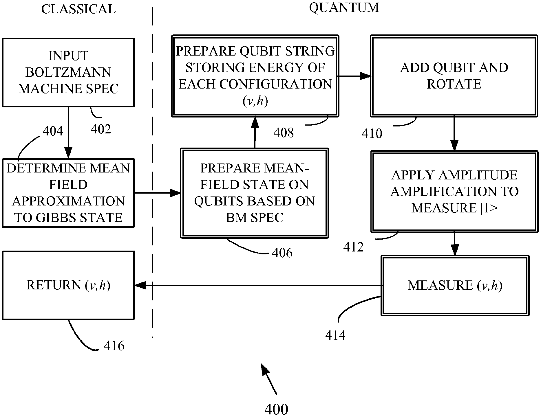
The disclosure provides methods and devices for training deep belief networks in machine learning. The disclosed methods allow for the efficient training of Boltzmann generic machines, which are currently not trainable using conventional approaches. The disclosed methods can also provide faster training with fewer steps. A quantum computer combined with a classic computer is used to determine the gradients of objective function for deep Boltzmann machine. Quantum states encode an approximate Gibbs distribution. A sampling of the approximate distribution is then used to determine Boltzmann biases and weights. In some cases, fast quantum algorithms and amplitude estimation are used. A classical computer will typically receive a Boltzmann Machine specification and training data and determine an objective function for the Boltzmann Machine. A quantum computer establishes at least one gradient for the objective function. Based on this gradient, the Boltzmann Machine is given at least one hidden weight or value. “A mean-field approximation may be used to define the objective function and gradients based on sampling can be determined.
The following features and others of the disclosure will be described with reference to the drawings.
As used in the present application and the claims, singular forms are?a? ?an,? The plural forms?an?,? Include the plural form unless the context clearly dictates that it is not. Also, the word ‘includes’ is used. means ?comprises.? The term “coupled” is also used to describe items that are “comprising”. The term “coupled” does not exclude intermediate elements that are present between the items.
The systems, apparatus and methods described in this document should not be construed to be restrictive. The present disclosure is aimed at all novel, non-obvious aspects and features of the disclosed embodiments alone, and in different combinations. The disclosed systems and methods are not restricted to any particular aspect or feature, or any combination thereof. Nor do they require any one or more advantages or problems to be resolved. “Any theories of operation will be used to explain the systems and methods disclosed, but they are not limited by them.
While the operations of certain disclosed methods are described sequentially for convenience, it is important to understand that this description includes rearrangement unless specific language below requires a particular order. In some cases, sequential operations can be rearranged and performed simultaneously. For simplicity’s sake, the figures attached may not depict the many ways that the disclosed systems and methods can be combined with other systems and methods. The description also uses words like “produce” and “provide”. The description of the disclosed methods sometimes uses terms like?produce? To describe the disclosed methods. These terms are abstractions at a high level of the actual operations performed. These terms are high-level abstractions of the actual operations performed.
In some examples, values or procedures are described as “lowest”, “best”, or “minimum”. Or something similar. These descriptions will help you to understand that they are meant to show that there are many options available and that these choices do not have to be superior, smaller or more desirable than other selections.
The methods and apparatus described in this document generally employ a classical computer coupled with a quantum computing device to train a Boltzmann deep machine. To update the model of the deep Boltzmann Machine, the classical computer must compute certain expectation values. This process is accelerated by a quantum computer. In most examples, an approximation of the state obtained by the mean-field approximation or another approximation is used to create a quantum state which is very close to the distribution resulting in the desired expectation value. This approximation is refined by the quantum computer into the exact distribution desired. By sampling this quantum distribution, the required expectation values can be learned.

In alternative examples, amplitude estimation is used. In order to obtain the required expectation values, instead of preparing the quantum computing system in a state that corresponds to a single vector of training, it is prepared as a quantum superposition based on all the training examples in the set. Amplitude estimation can be used for this.
Boltzmann Machines
The Boltzmann Machine is a powerful machine-learning paradigm in which the problem to train a system for classification or to generate examples from a set training vectors can be reduced to the energy minimization problem of a spinning system. The Boltzmann Machine is made up of binary units which are divided into two categories – visible units and hidden units. The visible units are those in which inputs and out put of the machine is given. If a machine is being used for classification then the visible unit will be used both to store training data and a label. The hidden units can be used to create correlations between visible units, allowing the machine to either assign a label to a training vector that is given or generate an example for the type of data the system has been trained to output. FIG. FIG. 1 shows a deep Boltzmann 100 machine that has a visible input 102 layer for inputs, an output layer 110 layer for outputs, and hidden unit layers (104,106,108) that connect the visible input 102 layer and the visible output 104 layer. Layers 102,104,106,108,110 can be connected with an adjacent layer by connections 103.105.107.109. However, in a machine like the one shown in FIG. There are no interlayer connections in FIG. “However, the disclosed methods can be used to teach Boltzmann machine with such intralayer connection, but for convenience, training deep Boltzmann devices is described in details.
Formally, the Boltzmann machine models the probability of a given configuration (v, h) of hidden and visible units via the Gibbs distribution:\nP(v,h)=e ?E(v,h) /Z\nwherein Z is a normalizing factor known as the partition function, and v,h refer to visible and hidden unit values, respectively. The energy E for a given combination of visible and hidden units has the following form:
E\n?\n(\nv\n,\nh\n)\n=\n?\ni\n?\nv\ni\n?\nb\ni\n-\n?\nj\n?\nh\nj\n?\nd\nj\n-\n?\ni\n,\nj\n?\nw\nij\n?\nv\ni\n?\nh\nj\n,
where vectors v, h, and vectors b, d, are the visible and hidden units, vectors, c, e, and f are the biases, which provide an energy penalty when a hit takes a value 1, and weight, wi,j, is a penalty that applies an energy penalty to both hidden and visible unit values of 1. The training of a Boltzmann device is reduced to estimating the biases and the weights using the training data. Boltzmann machines that have biases and/or weights determined are referred to as trained Boltzmann machines. To prevent overfitting and to obtain the following objective function, an L2-regularization can be used.
O\nML\n:=\n1\nN\ntrain\n?\n?\nv\n?\n?\nx\ntrain\n?\nlog\n(\n?\nh\n?\nP\n?\n(\nv\n,\nh\n)\n)\n-\n?\n2\n?\nw\nT\n?\nw\n.
This objective function is called a maximum-likelihood-objective (ML) function, and? Regularization is the term used to describe this function. Gradient descent is a way to find the locally optimal value for the ML-objective. The gradients for this objective function are written in the following way:
?\nO\nML\n?\nw\nij\n=\n?\nv\ni\n?\nh\nj\n?\ndata\n-\n?\nv\ni\n?\nh\nj\n?\nmodel\n-\n?\n?\n?\nw\ni\n,\nj\n(\n1\n?\na\n)\n?\nO\nML\n?\nb\ni\n=\n?\nv\ni\n?\ndata\n-\n?\nv\ni\n?\nmodel\n(\n1\n?\nb\n)\n?\nO\nML\n?\nd\nj\n=\n?\nh\nj\n?\ndata\n-\n?\nh\nj\n?\nmodel\n.\n(\n1\n?\nc\n)
The expectation values of a quantity x (v,h) can be calculated by:

?\nx\n?\ndata\n=\n1\nN\ntrain\n?\n?\nv\n?\nx\ntrain\n?\n?\nh\n?\nx\n?\n(\nv\n,\nh\n)\n?\ne\n-\nE\n?\n(\nv\n,\nh\n)\nZ\nv\n,\n?\nwherein\n?\n?\nZ\nv\n=\n?\nh\n?\ne\n-\nE\n?\n(\nv\n,\nh\n)\n,\nand\n?\nx\n?\nmodel\n=\n?\nv\n,\nh\n?\nx\n?\n(\nv\n,\nh\n)\n?\ne\n-\nE\n?\n(\nv\n,\nh\n)\nZ\n,\n?\nwherein\n?\n?\nZ\n=\n?\nv\n,\nh\n?\ne\n-\nE\n?\n(\nv\ndata\n,\nh\n)\n.

Click here to view the patent on Google Patents.


